Blog Home

NYC 311 Open Data

May 13, 2017

NYC Open Data includes data on 311 Service Requests.

I used at this dataset to look at complaint types:

over time
by month
by borough
time of day.

I looked at data from 2013 to May 2017.

Biggest Complaint

There were 275 different complaint types. The most frequent complaint during this time period was Residental Noise, with 848,649 complaints.

biggest_complaint <- as.data.frame(table(df_comb2$Complaint.Type))

biggest_complaint1 <- biggest_complaint %>%
                        arrange(desc(Freq))

## A tibble: 275 x 2
##                      Var1   Freq
##                    <fctr>  <int>
## 1     Noise - Residential 848649
## 2          HEAT/HOT WATER 688968
## 3        Street Condition 444825
## 4  Street Light Condition 404171
## 5        Blocked Driveway 401503
## 6         Illegal Parking 369456
## 7                 HEATING 300493
## 8                PLUMBING 276949
## 9            Water System 273922
## 10   UNSANITARY CONDITION 251285
## ... with 265 more rows

Complaints by Month

Heat/Hot Water was the biggest complaints for the winter months (Jan-March, Nov-Dec). Residential Noise was the biggest complaint for the other months, April to October.

January had the most complaints, and October had the least, from 2013 to May 2017.

month3.1 <- month1 %>%
              group_by(Var1, Var2) %>%
              summarise(freq  = sum(Freq)) %>%
              arrange(Var2, desc(freq))

    
tbl_df(month3.1)

month3.2 <- month3.1[!duplicated(month3.1$Var2), ]
    
tbl_df(month3.2)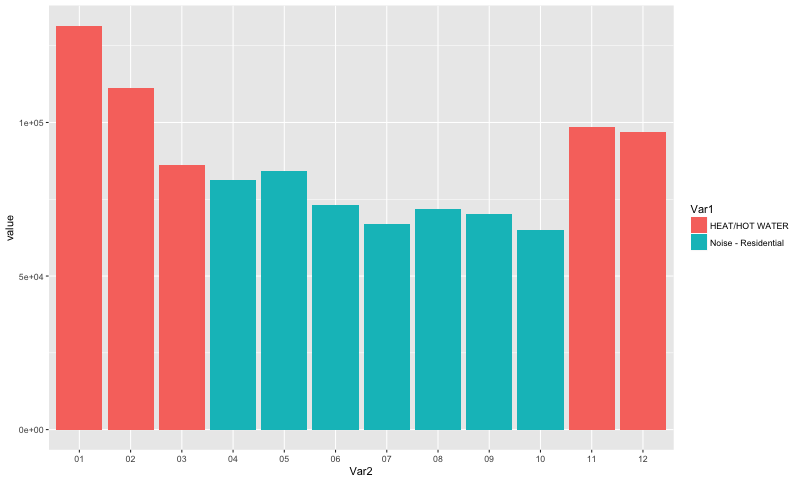

months_complaints

## A tibble: 12 x 4
##                  Var1   Var2 variable  value
##                <fctr> <fctr>   <fctr>  <int>
##1       HEAT/HOT WATER     01     freq 131518
##2       HEAT/HOT WATER     02     freq 111072
##3       HEAT/HOT WATER     03     freq  86287
##4  Noise - Residential     04     freq  81390
##5  Noise - Residential     05     freq  84272
##6  Noise - Residential     06     freq  73153
##7  Noise - Residential     07     freq  67008
##8  Noise - Residential     08     freq  71881
##9  Noise - Residential     09     freq  70231
##10 Noise - Residential     10     freq  64903
##11      HEAT/HOT WATER     11     freq  98520
##12      HEAT/HOT WATER     12     freq  96917

Time of day

Complaints were filed mostly in the morning in 2013 and 2014, but in 2015, 2016, and YTD 2017, complaints are filed more in the afternoon.

## Get complaint types by morning or afternoon

am_pm <- as.data.frame(table(df_comb2$am_pm1, df_comb2$year))

str(am_pm)

## Group by year and complaint type, and sum number of complaints

am_pm1 <- am_pm %>%
          group_by(Var1, Var2) %>%
          summarise(frequency = sum(Freq))

head(am_pm1)

am_pm1

## Plot complaints by time of day
ggplot(data=am_pm1, aes(x=Var2, y=frequency, fill=Var1)) + 
  geom_bar(stat="identity", position=position_dodge()) + theme(axis.text.x = element_text(angle = 45, hjust = 1))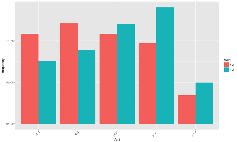

am.pm_complaints

Complaint with Biggest Increase

The complaint with the biggest percentage increase from 2013 to 2016 was Homeless Person Assistance, which increased by 9,923.5%, from 456 in 2013 to 45,707 complaint in 2016.

## Look at the number of each type of complaint per year
year.comp_type <- as.data.frame(table(df_comb2$year, df_comb2$Complaint.Type))

## Reshape from long to wide format
year.comp_type.long <- spread(year.comp_type, Var1, Freq)

## Get row sums (total for each complaint)

year.comp_type.long1$sum <- rowSums(year.comp_type.long1[2:6])

## Get percentage change of each complaint type, from 2013 to 2016
year.comp_type.long1$perc.change <- ((year.comp_type.long1$`2016` - year.comp_type.long1$`2013`)/year.comp_type.long1$`2013`) * 100

## Replace percentage changes of NaN with 0
year.comp_type.long1$perc.change <- gsub("NaN", "0", year.comp_type.long1$perc.change)
## Replace percentage changes of Inf with 1
year.comp_type.long1$perc.change <- gsub("Inf", "1", year.comp_type.long1$perc.change)

## Sort data descending by percentage change, and keep only the top five rows
year.comp_type.long_top5_percChange <- year.comp_type.long1 %>%
  arrange(desc(`perc.change`))%>%
  slice(1:5) %>%
  select(-`2017`, -sum)

## Reshape data from wide to long
year.comp_type.long_top5_percChange.long <- melt(year.comp_type.long_top5_percChange)

## Create bar chart showing change in complaint types over year, for complaint types with  five highest percentage changes 
ggplot(data=year.comp_type.long_top5_percChange.long, aes(x=variable, y=value, group= Var2, color= Var2)) +
  geom_line() +
  geom_point()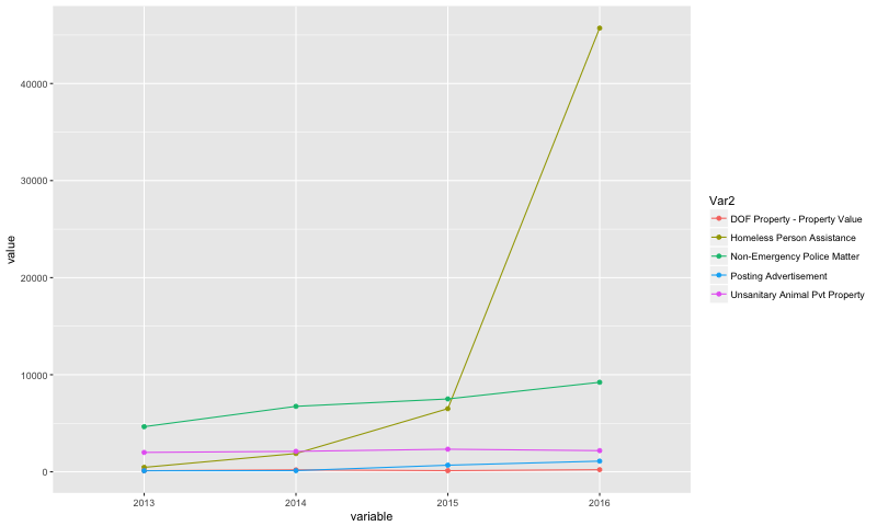

year_comparison

## A tibble: 5 x 6
##                             Var2  2013  2014  2015  2016      perc.change
##                           <fctr> <int> <int> <int> <int>            <chr>
## 1     Homeless Person Assistance   456  1883  6505 45707  9923.4649122807
## 2    Non-Emergency Police Matter  4648  6744  7506  9223 98.4294320137694
## 3  DOF Property - Property Value   110   199   119   216 96.3636363636364
## 4          Posting Advertisement   106   120   681  1100 937.735849056604
5##  Unsanitary Animal Pvt Property  1996  2108  2329  2181  9.2685370741483

Borough

Brooklyn had the most complaints, with 2,834,130 complaints, followed by Queens, Manhattan, the Bronx, and Staten Island.

complaint_borough_summary <- as.data.frame(table(df_comb2$Borough))

complaint_borough_summary1<- complaint_borough_summary %>%
                                arrange(desc(Freq))

tbl_df(complaint_borough_summary1)

# A tibble: 6 x 2
           Var1    Freq
         <fctr>   <int>
1      BROOKLYN 2834130
2        QUEENS 2079916
3     MANHATTAN 1971470
4         BRONX 1746389
5 STATEN ISLAND  444498
6   Unspecified  368803

The biggest complaints by borough were:

Residential Noise in Brooklyn and Manhattan (256,618 in Brooklyn, 196,582 in Manhattan);
Heat/Hot Water in the Bronx (225,871 complaints;
Blocked Driveway in Queens (164,471 complaints);
Streen condition in Staten Island (58,964 complaints)

Bronx

# Get frequency of each complaint type by borough

b1 <- as.data.frame(table(df_comb2$Borough, df_comb2$Complaint.Type))
b1

## Group and Sum
b2 <- b1 %>%
        group_by(Var1, Var2) %>%
        summarise(Frequency = sum(Freq))

b3 <- b2 %>%
        arrange(Var1, desc(Frequency))



## Get the Bronx's top five complaints, and add back in the number of those complaints for the other boroughs (the inner join)

b3_bronx1 <- b3 %>%
  filter(Var1=="BRONX") %>%
  arrange(desc(Frequency)) %>%
  slice(1:5) 

tbl_df(b3_bronx1)

b3_bronx <- b3 %>%
              filter(Var1=="BRONX") %>%
              arrange(desc(Frequency)) %>%
              slice(1:5) %>%
              inner_join(b2, by=c("Var2"))

## A tibble: 5 x 3
##    Var1                   Var2 Frequency
##  <fctr>                 <fctr>     <int>
##1  BRONX         HEAT/HOT WATER    225871
##2  BRONX    Noise - Residential    205636
##3  BRONX                HEATING    102574
##4  BRONX               PLUMBING     85879
##5  BRONX Street Light Condition     77134

Brooklyn

## Get Brooklyn's top five complaints, and add back in the number of those complaints for the other boroughs (the inner join)
b3_brooklyn <- b3 %>%
  filter(Var1=="BROOKLYN") %>%
  arrange(desc(Frequency)) %>%
  slice(1:5) %>%
  inner_join(b2, by=c("Var2"))

## Plot Brooklyn's top 5 complaints
ggplot(data=b3_brooklyn, aes(x=Var2, y=Frequency.y, fill=Var1.y)) + 
  geom_bar(stat="identity", position=position_dodge())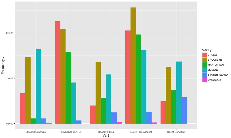

brooklyn_complaints

## A tibble: 5 x 3
##      Var1                Var2 Frequency
##    <fctr>              <fctr>     <int>
##1 BROOKLYN Noise - Residential    256618
##2 BROOKLYN      HEAT/HOT WATER    207894
##3 BROOKLYN    Blocked Driveway    146749
##4 BROOKLYN     Illegal Parking    135967
##5 BROOKLYN    Street Condition    124929

Manhattan

## Get Manhattan's top five complaints, and add back in the number of those complaints for the other boroughs (the inner join)
b3_manh <- b3 %>%
  filter(Var1=="MANHATTAN") %>%
  arrange(desc(Frequency)) %>%
  slice(1:5) %>%
  inner_join(b2, by=c("Var2"))

Queens

## Get Queen's top five complaints, and add back in the number of those complaints for the other boroughs (the inner join)

b3_queens <- b3 %>%
  filter(Var1=="QUEENS") %>%
  arrange(desc(Frequency)) %>%
  slice(1:5) %>%
  inner_join(b2, by=c("Var2"))

## A tibble: 5 x 3
##    Var1                   Var2 Frequency
##  <fctr>                 <fctr>     <int>
##1 QUEENS       Blocked Driveway    164471
##2 QUEENS    Noise - Residential    162566
##3 QUEENS       Street Condition    137251
##4 QUEENS Street Light Condition    127942
##5 QUEENS        Illegal Parking    108240

Staten Island

## Get Staten Island's top five complaints, and add back in the number of those complaints for the other boroughs (the inner join)
b3_si <- b3 %>%
  filter(Var1=="STATEN ISLAND") %>%
  arrange(desc(Frequency)) %>%
  slice(1:5) %>%
  inner_join(b2, by=c("Var2"))

Borough Comparison

## Combine all top 5's together


borough_top5 <- rbind(b3_bronx, b3_brooklyn, b3_manh, b3_queens, b3_si)

# borough_top5_1 <- borough_top5 %>%
#   inner_join(b2, by=c("Var2"))

## Plot all boroughs' top 5 complaints
ggplot(data=borough_top5_1, aes(x=Var2, y=Frequency.y, fill=Var1.y)) + 
  geom_bar(stat="identity", position=position_dodge()) + theme(axis.text.x = element_text(angle = 45, hjust = 1)) + facet_grid(Var1.y ~. )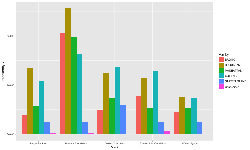

all_boroughs

Get Data!

To get the data summarized above, here is the set up.

library(RCurl) 
library(dplyr)
library(stringr)
library(reshape)
library(tidyr)
library(ggplot2)

## Read Files
df2017ytd <- read.csv("311_Service_Requests_from_2010_to_Present (2).csv")
df2016 <- read.csv("311_Service_Requests_from_2010_to_Present.csv")
df2013 <- read.csv("311_Service_Requests_from_2013.csv")
df2014 <- read.csv("311_Service_Requests_from_2014 2.csv")
df2015 <- read.csv("311_Service_Requests_from_2015.csv")

## Combine Files
df_comb <- rbind(df2014,df2015, df2016, df2017ytd)
df_comb1 <-rbind(df_comb, df2013)

## Split date column to month, day, year, time, and AM/PM
df_comb1$month <- sapply(strsplit(as.character(df_comb1$Created.Date),'/'), "[", 1)
df_comb1$day <- sapply(strsplit(as.character(df_comb1$Created.Date),'/'), "[", 2)
df_comb1$year <- sapply(strsplit(as.character(df_comb1$Created.Date),'/'), "[", 3)

df_comb1$time <- sapply(strsplit(as.character(df_comb1$Created.Date),' '), "[", 1)
df_comb1$am_pm <- sapply(strsplit(as.character(df_comb1$Created.Date),' '), "[", 2)
df_comb1$am_pm1 <- sapply(strsplit(as.character(df_comb1$Created.Date),' '), "[", 3)

## Get only columns needed

df_comb2 <- df_comb1[c(1:9,17,19,25,54:57,59:60)]

## Replace NA's to 0's
df_comb2[is.na(df_comb2)] <- 0

## A tibble: 9,445,206 x 18
##   Unique.Key           Created.Date            Closed.Date Agency
##*       <int>                 <fctr>                 <fctr> <fctr>
##1    28457271 07/11/2014 03:08:58 PM 08/05/2014 12:41:37 PM    DOT
##2    28644314 08/08/2014 02:06:22 PM 08/12/2014 11:33:34 AM    DCA
##3    29306886 11/18/2014 12:52:40 AM 11/18/2014 01:35:22 AM   NYPD
##4    28907593 09/18/2014 01:45:51 PM 09/22/2014 02:43:43 PM   FDNY
##5    28908228 09/18/2014 06:43:00 PM 09/18/2014 06:43:57 PM    HRA
##6    29423275 12/04/2014 12:45:08 AM 12/04/2014 07:22:41 AM   NYPD
##7    29419044 12/03/2014 02:08:52 PM 12/03/2014 05:23:13 PM   NYPD
##8    27768554 04/02/2014 07:46:56 PM 04/03/2014 08:00:27 AM    DOT
##9    28254593 06/13/2014 03:17:13 PM 07/22/2014 12:22:11 PM  DOHMH
##10   27982973 05/05/2014 11:42:00 AM 05/12/2014 10:47:32 AM    DOT
### ... with 9,445,196 more rows, and 14 more variables: Agency.Name <fctr>, Complaint.Type <fctr>,
###   Descriptor <fctr>, Location.Type <fctr>, Incident.Zip <fctr>, City <fctr>, Facility.Type <fctr>,
###   Borough <fctr>, month <chr>, day <chr>, year <chr>, time <chr>, am_pm <chr>, am_pm1 <chr>

Nadine Khattak Fischoff