Blog Home

Using R to Map NYC and SF 311 Service Requests

Jun 5, 2017

Google BigQuery has public datasets with up-to-date data on 311 Service Request for both San Francisco (starting in 2008) and NYC (starting in 2010).

I did some comparisons between the top complaints between both cities, and not surprisingly, they were very different. NYC’s top complaints are for heat/hot water, especially in the winter months; and San Francisco’s top complaints are for disposal of bulky items, and general cleaning. This post won’t go into detail on the differences. Instead here, I map the frequency of complaints for the top complaint in each city in 2016.

Here are the two maps, and below that, explanations of how I created each map.

sf_bi

ny_hhw

San Francisco

Top Complaints

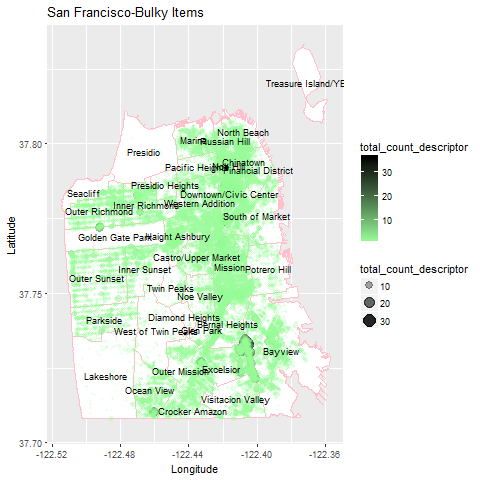
The top complaint in SF in 2016 was for Bulky Item recycling.

SQL query:

#standardSQL
SELECT
complaint_type,
COUNT(descriptor) AS total_count
FROM
`bigquery-public-data.san_francisco.311_service_requests`
WHERE
EXTRACT(year from created_date) = 2016
GROUP BY complaint_type
ORDER BY
2 DESC

I read in the data, and took a look at just the top 10 complaints:

top2016SF <- read.csv("top2016SF.csv")

top2016SF_10 <- top2016SF %>%
                  slice(1:10) %>%
                  rename(c('total_count_descriptor' = 'total_count'))

Here are the top 10 complaints by frequency in SF during 2016:

# A tibble: 10 x 2
#                                     complaint_type total_count
#                                             <fctr>       <int>
# 1                                      Bulky Items       70243
# 2                                 General Cleaning       54622
# 3                               Encampment Reports       26930
# 4                                      Human Waste       18568
# 5                              request_for_service       15101
# 6                  Graffiti on Building_commercial       10073
# 7                                        complaint        9303
# 8                                 Graffiti on Pole        8308
# 9                                  Pavement_Defect        7926
#10 Graffiti on Other_enter_additional_details_below        7559

If you’re like me, you might be wondering what exactly the “Bulky Items” are. We can grab another column, descriptors and get some details.

Here is the SQL Query:

#standardSQL
SELECT
complaint_type,
descriptor,
COUNT(descriptor) AS total_count_descriptor
FROM
`bigquery-public-data.san_francisco.311_service_requests`
WHERE
complaint_type = "Bulky Items"
and EXTRACT(year from created_date) = 2016
GROUP BY complaint_type, descriptor
ORDER BY
2 DESC

Read in the results:

b_desc <- read.csv("D:/sfnyc/bulky_items_desc.csv")
b_desc <- b_desc %>%
            arrange(desc(total_count_descriptor))

Display results:

# A tibble: 5 x 3
#  complaint_type            descriptor total_count_descriptor
#          <fctr>                <fctr>                  <int>
#1    Bulky Items             Furniture                  23823
#2    Bulky Items Boxed or Bagged Items                  21476
#3    Bulky Items              Mattress                  10780
#4    Bulky Items          Refrigerator                   9467
#5    Bulky Items           Electronics                   4697

People called 311 in San Francisco mainly for recycling or disposal of furniture and boxed or bagged items.

Mapping the Top Complaints

Get Data

I ran a SQL query getting the 2016 count of Bulky Item complaints by location (latitude and longitude).

I had to split this up into different segments based on months, because Google BigQuery wouldn’t allow me to download CSV’s that were more than 16,000 rows. Another way to do this would have been to get the total, and split up the rows into 16,000 rows each, by using LIMIT 16000 OFFSET 16000.

#standardSQL
SELECT
complaint_type,
longitude,
latitude,
COUNT(descriptor) AS total_count_descriptor
FROM
`bigquery-public-data.san_francisco.311_service_requests`
WHERE
complaint_type = "Bulky Items"
and EXTRACT(year from created_date) = 2016
and EXTRACT(month from created_date) < 3
and longitude != 0
GROUP BY complaint_type, descriptor,longitude, latitude
ORDER BY
2 DESC

I read in the separate files with R, combined them together, and sorted descending by count of complaints.

sfb1 <- read.csv("sfmo_lt3.csv")
sfb2 <- read.csv("sfmo_gte3.lt6.csv")
sfb3 <- read.csv("sfmo_gte6.lt9.csv")
sfb4 <- read.csv("sfmo_gte9.lte12.csv")
sfb5 <- read.csv("mosf_e12month.csv")

sfba <- rbind(sfb1, sfb2, sfb3, sfb4, sfb5)


sfba <- sfba %>%
          arrange(desc(total_count_descriptor))

Here is sample of the sfba dataframe:

# A tibble: 60,045 x 4
#   complaint_type longitude latitude total_count_descriptor
#           <fctr>     <dbl>    <dbl>                  <int>
# 1    Bulky Items -122.4059 37.73296                     36
# 2    Bulky Items -122.4090 37.73129                     31
# 3    Bulky Items -122.4059 37.73296                     30
# 4    Bulky Items -122.4185 37.77483                     30
# 5    Bulky Items -122.4059 37.73296                     30
# 6    Bulky Items -122.4185 37.77483                     26
# 7    Bulky Items -122.4185 37.77483                     25
# 8    Bulky Items -122.4059 37.73296                     24
# 9    Bulky Items -122.4185 37.77483                     24
#10    Bulky Items -122.4047 37.73032                     23
# ... with 60,035 more rows

Create Map

The next step is map the the complaints and show areas where complaints are more frequent.

I got the shapefile for San Francisco from the ArcGIS.

I read this shapefile data with R, and converted the coordinates to longitudes and latitudes.

ba <-readOGR("D:/pn","planning_neighborhoods")
ba_wgs84 <- spTransform(ba, CRS("+proj=longlat +datum=WGS84"))

ba_wgs84@data$id = rownames(ba_wgs84@data)
ba_wgs84.points = fortify(ba_wgs84, region="id")
ba_wgs84.df = join(ba_wgs84.points, ba_wgs84@data, by="id")

tbl_df(ba_wgs84.df)

Here is what that ends up looking like:

> tbl_df(ba_wgs84.df)

# A tibble: 13,254 x 8
#        long      lat order  hole  piece    id  group neighborho
#       <dbl>    <dbl> <int> <lgl> <fctr> <chr> <fctr>     <fctr>
# 1 -122.4841 37.78791     1 FALSE      1     0    0.1   Seacliff
# 2 -122.4843 37.78765     2 FALSE      1     0    0.1   Seacliff
# 3 -122.4874 37.78749     3 FALSE      1     0    0.1   Seacliff
# 4 -122.4871 37.78376     4 FALSE      1     0    0.1   Seacliff
# 5 -122.4925 37.78350     5 FALSE      1     0    0.1   Seacliff
# 6 -122.4924 37.78166     6 FALSE      1     0    0.1   Seacliff
# 7 -122.5053 37.78100     7 FALSE      1     0    0.1   Seacliff
# 8 -122.5051 37.77977     8 FALSE      1     0    0.1   Seacliff
# 9 -122.5062 37.77987     9 FALSE      1     0    0.1   Seacliff
#10 -122.5078 37.77995    10 FALSE      1     0    0.1   Seacliff
# ... with 13,244 more rows

I then get a list of the neighborhoods and their coordinates, to use as map labels:

baidList <- ba_wgs84@data$neighborho
centroids.df <- as.data.frame(coordinates(ba_wgs84))
names(centroids.df) <- c("Longitude", "Latitude")  #more sensible column names
id.df <- data.frame(id = baidList, centroids.df)

And that looks like this:

> tbl_df(id.df)

# A tibble: 37 x 3
#                      id Longitude Latitude
# *                <fctr>     <dbl>    <dbl>
# 1              Seacliff -122.5011 37.78382
# 2        Haight Ashbury -122.4463 37.76929
# 3         Outer Mission -122.4441 37.72411
# 4          Russian Hill -122.4185 37.80116
# 5            Noe Valley -122.4333 37.74935
# 6          Inner Sunset -122.4654 37.75849
# 7 Downtown/Civic Center -122.4160 37.78335
# 8       Diamond Heights -122.4425 37.74231
# 9   Treasure Island/YBI -122.3695 37.82066
#10             Lakeshore -122.4886 37.72260
# ... with 27 more rows

I put it all together with the map and points showing where the complaints were made, and the frequency of the complaints. The geom_point(aes(color=total_count_descriptor, size=total_count_descriptor, alpha=total_count_descriptor) ) code makes this more of a heat map, rather than just points on the map.

Coordinates with several complaints have larger, darker plots, and coordinates with fewer complaints are green, smaller, and less opaque.

chart2 <- ggplot(sfba, aes(longitude, latitude))  + #"id" is col in your df, not in the map object
  expand_limits(x = ba_wgs84.df$long, y = ba_wgs84.df$lat) +
  geom_polygon(data= ba_wgs84.df, aes(x=long, y=lat, group=group), fill="white", color="pink", size=0.15) +
  geom_point(aes(color=total_count_descriptor, size=total_count_descriptor, alpha=total_count_descriptor) ) +
  geom_text(data=id.df, aes(label = id, x = Longitude, y = Latitude), size = 1.5) +
  labs(x = "Longitude", y = "Latitude", title = "CTE") +
   scale_colour_gradient(low = "#99ff99", high = "black")

sf_bi

The downtown SF areas had a high density of calls, and Bayview had specific locations with several bulky item complaints, as shown with the larger, darker circles.

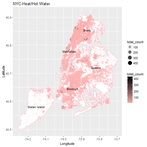
New York city

I went through the same process to get the map for NYC. I got the NYC borough shapefile from NYC Planning.

The BigQuery table for the NYC 311 data is bigquery-public-data.new_york.311_service_requests.

Here are the results of the same queries and tables created with R, for NYC.

Top 2016 Complaints

# A tibble: 10 x 2
#            complaint_type total_count
#                    <fctr>       <int>
# 1          HEAT/HOT WATER      227959
# 2     Noise - Residential      221906
# 3         Illegal Parking      122479
# 4        Blocked Driveway      119046
# 5        Street Condition       90674
# 6  Street Light Condition       89122
# 7    UNSANITARY CONDITION       80469
# 8            Water System       73368
# 9 Noise - Street/Sidewalk       61199
#10           PAINT/PLASTER       60336

Heat/Hot Water descriptors

# A tibble: 2 x 3
  complaint_type      descriptor total_count_descriptor
          <fctr>          <fctr>                  <int>
1 HEAT/HOT WATER ENTIRE BUILDING                 150114
2 HEAT/HOT WATER  APARTMENT ONLY                  77845

Ten Locations with Most Complaints

# A tibble: 71,268 x 4
   complaint_type longitude latitude total_count
           <fctr>     <dbl>    <dbl>       <int>
 1 HEAT/HOT WATER -73.87685 40.74742         421
 2 HEAT/HOT WATER -73.87685 40.74742         386
 3 HEAT/HOT WATER -73.87730 40.82459         362
 4 HEAT/HOT WATER -73.92715 40.86194         307
 5 HEAT/HOT WATER -73.92715 40.86194         299
 6 HEAT/HOT WATER -73.87685 40.74742         290
 7 HEAT/HOT WATER -73.97488 40.78507         270
 8 HEAT/HOT WATER -74.00856 40.63490         266
 9 HEAT/HOT WATER -73.87730 40.82459         263
10 HEAT/HOT WATER -73.87685 40.74742         258

Map with Locations of 2016 Complaints for Heat/Hot WATER