Blog Home
A Look at Hacker News Data
I decided to take a look at Hacker News data on Google BigQuery. This post gave me ideas of data to pull, and an idea of the type of SQL queries I could run.
I pulled the data with SQL queries, and used R to take a longitudinal look at domains with the most stories, from 2006 to 2017 year-to-date.And I used R’s TidyText package to do a pretty terse sentiment analysis of story titles for top stories by score; and again used the method from this post.
Domains with Most Stories, 2006 to May 2017
I got count of stories by domain for each year, from 2006 to 2017 year-to-date.
 SELECT
 REGEXP_EXTRACT(url, '//([^/]*)/?') domain
 , COUNT(*) c

 FROM `bigquery-public-data.hacker_news.full`
 WHERE url!=''
 GROUP BY domain ORDER BY c desc LIMIT 10
I read in the data :
fj3.1 <- read.csv("results-20170527-004428.csv")A look at the resulting dataframe:
> tbl_df(fj3.1)

# A tibble: 10 x 2
                domain     c
                <fctr> <int>
1           github.com 55751
2           medium.com 47725
3      www.youtube.com 45760
4       techcrunch.com 31056
5      www.nytimes.com 30675
6      arstechnica.com 18685
7        www.wired.com 14684
8     en.wikipedia.org 11874
9        www.bbc.co.uk 10968
10 www.theguardian.com 10705
Here’s a bar chart of the top 10 domains, from 2006 to 5/25/2017, by story count:
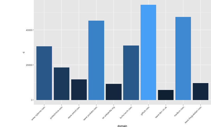
Github had the most stories submitted, with 55,751 stories submitted. Medium and Youtube were close behind. The Top five all are pretty close in story count. There’s a big drop-off after the top 5 (after the NY Times), with arstechnica.com having 49% (11,990) fewer stories than the NY Times.
Most Popular 2017 Domains and Change over Time
I looked at the 2017 YTD (May 2017) top 10 domains in Hacker News by count of stories, and how these domains have compared in the previous years, beginning with 2017.
First I ran this query to get the count of stories by the ten most popular domains in 2017.
standardSQL
 SELECT
 REGEXP_EXTRACT(url, '//([^/]*)/?') domain
 , COUNT(*) c
 , EXTRACT(YEAR FROM timestamp) y
 FROM `bigquery-public-data.hacker_news.full`
 WHERE url!='' AND EXTRACT(YEAR FROM timestamp) = 2006
 GROUP BY domain, y ORDER BY c desc LIMIT 10
Then I read in the results.
f2017 <- read.csv("results-20170522-132414.csv")Here is a look at the results:
tbl_df(f1)

# A tibble: 10 x 3
                domain     c     y
                <fctr> <int> <int>
1           medium.com  7388  2017
2           github.com  6384  2017
3      www.youtube.com  3836  2017
4      www.nytimes.com  2357  2017
5       techcrunch.com  1676  2017
6    www.bloomberg.com  1495  2017
7      arstechnica.com  1320  2017
8  www.theguardian.com  1306  2017
9             youtu.be  1099  2017
10    www.theverge.com  1013  2017
I then pulled the counts for each of these ten domains, by year.
 SELECT
 REGEXP_EXTRACT(url, '//([^/]*)/?') domain
 , COUNT(*) c
 , EXTRACT(YEAR FROM timestamp) y
 FROM `bigquery-public-data.hacker_news.full`
 WHERE REGEXP_EXTRACT(url, '//([^/]*)/?') in ('medium.com', 'github.com', 'www.youtube.com', 'www.nytimes.com', 'techcrunch.com', 'www.bloomberg.com', 'arstechnica.com',
                                              'www.theguardian.com', 'youtu.be', 'www.theverge.com')
 GROUP BY domain, y ORDER BY c desc
I read in the data and arranged it ascending by year.
fj2 <- read.csv("results-20170522-133430.csv")

fj2 <- fj2 %>%
          arrange(y)

fj2
Here are some of the results:
# A tibble: 90 x 3
              domain     c     y
              <fctr> <int> <int>
1    www.nytimes.com     9  2006
2    www.nytimes.com   474  2007
3    arstechnica.com   122  2007
4    www.youtube.com    99  2007
5  www.bloomberg.com    12  2007
6    www.nytimes.com  1650  2008
7    arstechnica.com   534  2008
8    www.youtube.com   326  2008
9  www.bloomberg.com    99  2008
10        github.com    66  2008
This line chart shows the change in count of stories by each top 10 2017 domain, from 2006 to May 2017.
ggplot(data=fj2, aes(x=y, y=c, group=domain, colour=domain)) +
  geom_line() +
  geom_point()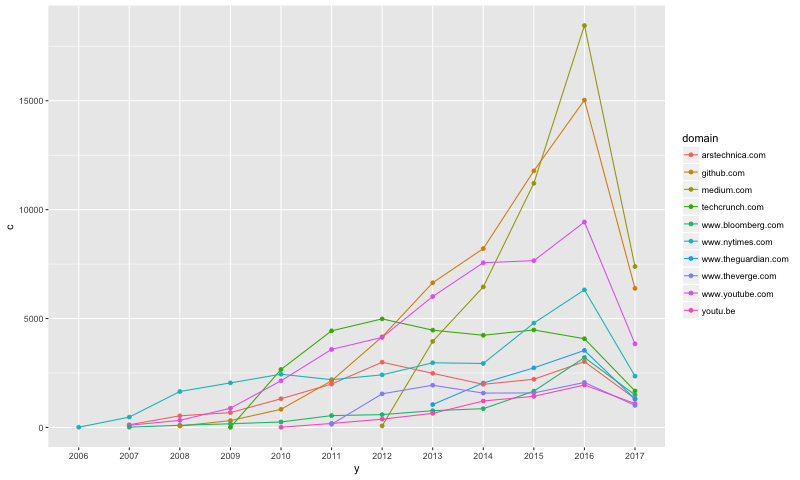
Sentiment Analysis on Top Stories’ Titles by Score
I then pulled the top 100 stories by score for each year, and used the TidyText package to compare sentiments expressed in the top stories for each year.
It looks like more negative emotions of anger and fear have shown increases in 2017 compared to other years, and negative sentiments are already higher not even halfway through the year, than they were in 2016. Negative sentiments in top story titles are higher in 2017 than in all of the previous years. Positive sentiments, on the other hand, are the least in 2017 compared to all other years.
First, I ran this SQL query for each year from 2006 to 2017:
 SELECT title
 ,score
 ,EXTRACT(YEAR FROM timestamp) year
 FROM  `bigquery-public-data.hacker_news.full`
 WHERE type = "story" and EXTRACT(YEAR FROM timestamp) = 2006 --> update year
 ORDER BY score desc
 LIMIT 100
I then read in the data:
s2017 <- read.csv("results-20170522-135935.csv")
s2016 <- read.csv("results-20170522-135950.csv")tbl_df(s2016)
s2015 <- read.csv("results-20170522-135957.csv")
s2014 <- read.csv("results-20170522-140005.csv")
s2013 <- read.csv("results-20170522-140012.csv")
s2012 <- read.csv("results-20170522-140019.csv")
s2011 <- read.csv("results-20170522-140026.csv")
s2010 <- read.csv("results-20170522-140035.csv")
s2009 <- read.csv("results-20170522-140044.csv")
s2008 <- read.csv("results-20170522-140053.csv")
s2007 <- read.csv("results-20170522-140100.csv")
s2006 <- read.csv("results-20170522-140109.csv")
I then got the list of words and their associated sentiments and emotions from the TidyText package:
nrc <- sentiments %>%
  filter(lexicon == "nrc") %>%
  dplyr::select(word, sentiment)
I then got only the words from the titles for each included story, for each year. Then I joined this table with the nrc dataframe, to associate each word included with the NRC sentiment/emotion table. I then counted the number of words associated with each sentiment/emotion.
s06 <- s2006 %>%
  filter(!str_detect(title, '^"')) %>%
  unnest_tokens(word, title, token = "regex") %>%
  filter(!word %in% stop_words$word,
         str_detect(word, "[a-z]")) %>%
  data.frame()

s06_1 <- s06 %>%
  inner_join(nrc, by = "word")
I did this for each year, and combined them into one dataframe, joining on sentiment.
sall_1 <- s06_2 %>%
            inner_join(s07_2, by="x") %>%
            inner_join(s08_2, by="x") %>%
            inner_join(s09_2, by="x") %>%
            inner_join(s10_2, by="x") %>%
            inner_join(s11_2, by="x") %>%
            inner_join(s12_2, by="x") %>%
            inner_join(s13_2, by="x") %>%
            inner_join(s14_2, by="x") %>%
            inner_join(s15_2, by="x") %>%
            inner_join(s16_2, by="x") %>%
            inner_join(s17_2, by="x")

names(sall_1)[2] <- '2006'
names(sall_1)[3] <- '2007'
names(sall_1)[4] <- '2008'
names(sall_1)[5] <- '2009'
names(sall_1)[6] <- '2010'
names(sall_1)[7] <- '2011'
names(sall_1)[8] <- '2012'
names(sall_1)[9] <- '2013'
names(sall_1)[10] <- '2014'
names(sall_1)[11] <- '2015'
names(sall_1)[12] <- '2016'
names(sall_1)[13] <- '2017'
Here is what the data looks like:
> tbl_df(sall_1)
# A tibble: 9 x 13
             x  2006  2007  2008  2009  2010  2011  2012  2013  2014  2015  2016
         <chr> <int> <int> <int> <int> <int> <int> <int> <int> <int> <int> <int>
1        anger     2     7     9     8    14    11    17    11    14     5     6
2 anticipation    13    16    20    16    20    11     9     8    13    11    14
3         fear     2     8    11     9    12    16    15    20    15    11    13
4          joy     7    13    13     9    10     2     7     7     5     7    15
5     negative     4    14    19    23    20    23    25    25    22    16    26
6     positive    21    38    31    29    28    23    21    26    26    23    44
7      sadness     1     5    11    11     9    15    14    11    12     4    17
8     surprise     8     4     7     6     7     5     3     4     5     2     6
9        trust    10    29    19    18    20    17    13    20    11    15    26
# ... with 1 more variables: 2017 <int>
I reshaped the data from wide to long format to create a bar chart:
sall_2 <- melt(sall_1)

sall_2 <- sall_2 %>%
            arrange(x)
# A tibble: 108 x 3
x variable value
<chr> <fctr> <int>
1 anger 2006 2
2 anger 2007 7
3 anger 2008 9
4 anger 2009 8
5 anger 2010 14
6 anger 2011 11
7 anger 2012 17
8 anger 2013 11
9 anger 2014 14
10 anger 2015 5
# ... with 98 more rowsThis bar chart creates a face for each sentiment, with one bar for each year:
ggplot(data=sall_2, aes(x=variable, y=value, fill=variable)) +
  geom_bar(stat="identity", position=position_dodge()) + theme(axis.text.x = element_text(angle=45, hjust=1)) +
  theme(plot.margin = unit(c(0,0,0,3), "cm")) + facet_grid( x ~ .)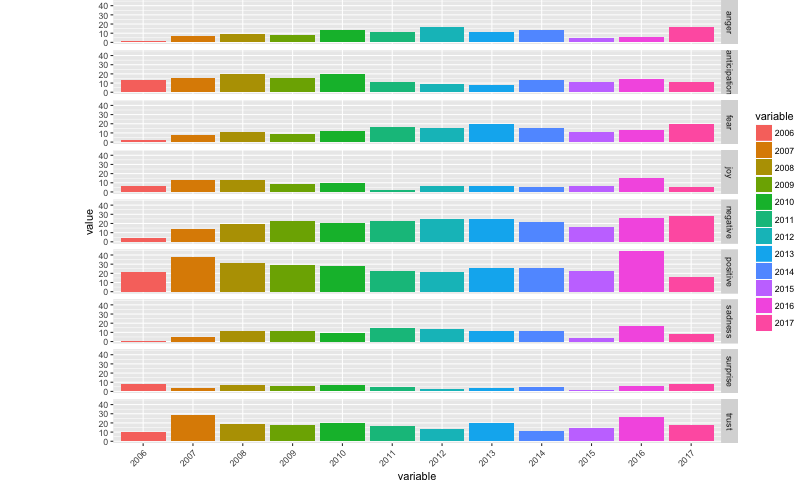
This stacked bar chart groups each sentiment onto one rung of the x axis, by year.
ggplot(data=sall_2, aes(x=x, y=value, fill=variable)) +
  geom_bar(stat="identity", position=position_dodge()) + theme(axis.text.x = element_text(angle=45, hjust=1)) +
theme(plot.margin = unit(c(0,0,0,3), "cm")) 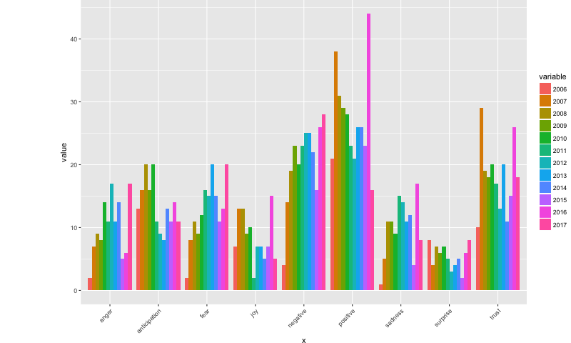
I then wanted to see if there was a difference in sentiments between the bottom 10 of the top 100 for each year, and the top ten scores for each year, from 2006 to 2017.
First, I took the top 10 from the top 100 for each year:
a1 <- s2006 %>%
        arrange(desc(score)) %>%
        slice(1:10)
I did this for each year, and combined them:
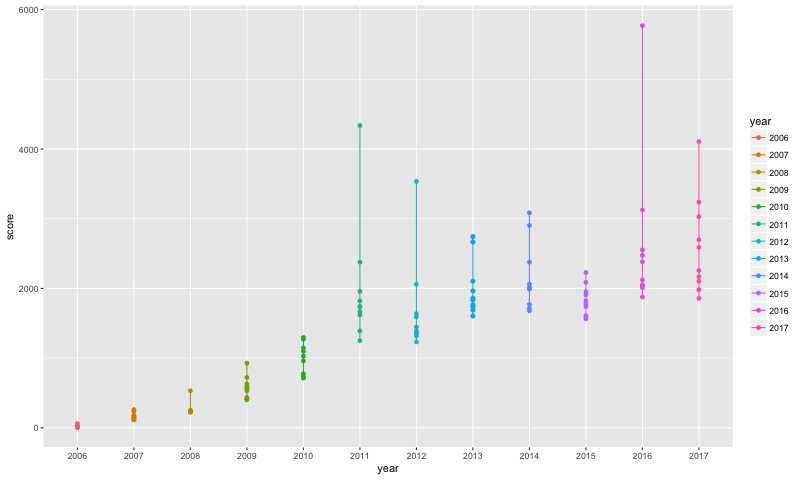
a14 <- rbind(a1, a2, a3, a4, a5, a6, a7, a8, a9, a10, a11, a12, a13)Because I now had the top ten stories by score for each year, I graphed it to see what the score range was for each year in the dataset.
a15 <- a14[c(2,3)]> tbl_df(a15)
# A tibble: 130 x 2
score year
* <int> <fctr>
1 61 2006
2 16 2006
3 12 2006
4 12 2006
5 11 2006
6 10 2006
7 9 2006
8 9 2006
9 8 2006
10 7 2006
# ... with 120 more rows
> The biggest range was in 2016, and the second-biggest range was in 2011.
I then did got the words out of the top 10 stories by score for each year, and merged that with the NRC dataset, and counted the sentiments for these stories.
a16 <- a14 %>%
  filter(!str_detect(title, '^"')) %>%
  unnest_tokens(word, title, token = "regex") %>%
  filter(!word %in% stop_words$word,
         str_detect(word, "[a-z]")) %>%
  data.frame()

a17 <- a16 %>%
  inner_join(nrc, by = "word")

a17_1 <- count(a17$sentiment)

a17_1$perc_top <- a17_1$freq / sum(a17_1$freq)
# A tibble: 10 x 3
x freq perc_top
<fctr> <int> <dbl>
1 anger 15 0.09803922
2 anticipation 13 0.08496732
3 disgust 12 0.07843137
4 fear 16 0.10457516
5 joy 6 0.03921569
6 negative 28 0.18300654
7 positive 27 0.17647059
8 sadness 14 0.09150327
9 surprise 3 0.01960784
10 trust 19 0.12418301I then got the bottom ten scores for each year:
b1 <- s2006 %>%
  arrange(score) %>%
  slice(1:10)
I did this for each year, then combined them; and then I merged these bottom ten with the top ten for each year.
b14 <- rbind(b1, b2, b3, b4, b5, b6, b7, b8, b9, b10, b11, b12, b13)I looked at the range for these bottom ten out of the top 100 stories by score. The range is much smaller than that for the top stories by score:
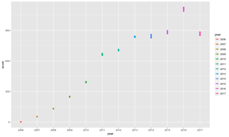
I then got just the words out of the titles of the stories, merged those words with the NRC datasets to get the sentiment/emotion for each word, and counted the number of words for each sentiment/emotion.
b16 <- b14 %>%
  filter(!str_detect(title, '^"')) %>%
  unnest_tokens(word, title, token = "regex") %>%
  filter(!word %in% stop_words$word,
         str_detect(word, "[a-z]")) %>%
  data.frame()

b17 <- b16 %>%
  inner_join(nrc, by = "word")

b17

b17_1 <- count(b17$sentiment)

b17_1

b17_1$perc_bottom <- b17_1$freq / sum(b17_1$freq)

sum(b17_1$perc_bottom)
> tbl_df(b17_1)
# A tibble: 10 x 3
x freq perc_bottom
<fctr> <int> <dbl>
1 anger 20 0.09478673
2 anticipation 17 0.08056872
3 disgust 13 0.06161137
4 fear 17 0.08056872
5 joy 14 0.06635071
6 negative 31 0.14691943
7 positive 39 0.18483412
8 sadness 14 0.06635071
9 surprise 9 0.04265403
10 trust 37 0.17535545I combined the a17_1 dataframe with the sentiments for the top ten stories, with the b17_1 dataframe, with the sentiments for the bottom ten out of the top 100 stories.
I reshaped the data to be able to create the bar chart comparing the sentiments between the two stories.
ab1 <- a17_1 %>%
        inner_join(b17_1, by="x")
ab1

ab1_1 <- ab1[c(1,3,5)]

ab2 <- melt(ab1_1)

ab2

ab2$variable <-  gsub('perc_top', 'top_10',ab2$variable )
ab2$variable <-  gsub('perc_bottom', 'bottom_10',ab2$variable )
# A tibble: 20 x 3
x variable value
<fctr> <chr> <dbl>
1 anger top_10 0.09803922
2 anticipation top_10 0.08496732
3 disgust top_10 0.07843137
4 fear top_10 0.10457516
5 joy top_10 0.03921569
6 negative top_10 0.18300654
7 positive top_10 0.17647059
8 sadness top_10 0.09150327
9 surprise top_10 0.01960784
10 trust top_10 0.12418301
11 anger bottom_10 0.09478673
12 anticipation bottom_10 0.08056872
13 disgust bottom_10 0.06161137
14 fear bottom_10 0.08056872
15 joy bottom_10 0.06635071
16 negative bottom_10 0.14691943
17 positive bottom_10 0.18483412
18 sadness bottom_10 0.06635071
19 surprise bottom_10 0.04265403
20 trust bottom_10 0.17535545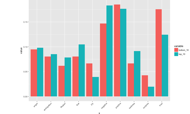
It looks like the top 10 stories were more negative and had more negative emotions than the bottom ten out of the top 100 stories.
The top 10 stories were higher in anger, anticipation, disgust, fear, and sadness. It was higher in the negative sentiments.
The bottom 10 stories were higher in positive sentiments and emotions of joy, surprise, and trust.